Earlier this month, Snowflake’s Customer Enablement Team was assigned an email from one of our customers. The customer stated that he was not happy about the idea of cloning full copies of production databases for development purposes. “Do we really want to develop and maintain a system to copy a fraction of the production DB to dev?”, citing the reason for his message that, by just copying the entire production database, the dev team would have access to too much data. Being a veteran of Snowflake, I initially dismissed his concern because of Snowflake’s zero-copy clone capability, as outlined in this article. From my perspective, the zero-copy clone would not incur any additional cost for development purposes, so why not give the dev team all of the data?
The answer of course, as the customer pointed out, has to do with making the development effort more efficient. The assumption of zero-copy clone equating to zero-cost development is, of course, incorrect. There’s the cost of querying the data (requiring virtual warehouse credits) and the cost behind each development hour. After all, longer query times lead to longer development iterations and longer testing cycles. To create a “blissful” development environment in Snowflake, we need a more refined approach towards building the development data set.
The approach outlined by the customer was rooted in complimenting Snowflake’s zero-copy clone with the additional technique of using Block Sampling. In other words, they proposed creating a view containing a sample set from the original table. This approach enables an administrator to quickly set up a dev environment with minimal data. Controlling the amount of sample data is a good thing for many development situations because developers seldom require access to the full dataset.
Ok, let’s take a look at SAMPLE / TABLESAMPLE and see how we can do this. The syntax is quite simple:
SELECT ...
FROM ...
 { SAMPLE | TABLESAMPLE } [ samplingMethod ] ( <probability> ) [ { REPEATABLE | SEED } ( <seed> ) ]
[ ... ]

-- Where:
  samplingMethod :: = { { BERNOULLI | ROW } | { SYSTEM | BLOCK } }
Note that there are some interchangeable terms we should pay attention to when writing the query. These terms are synonyms and only differ in syntax:
SAMPLE | TABLESAMPLE

BERNOULLI | ROW

SYSTEM | BLOCK

REPEATABLE | SEED
The two main methods of sampling are ROW (or BERNOULLI) and BLOCK (or SYSTEM) sampling. Let’s take a closer look at each one.
Row Sampling
This approach uses the Bernoulli principle to select data by applying a probability of p/100 to each row. In the Snowflake documentation, we mention that this is similar to “flipping a weighted coin” on each row. The number of sampled (selected) rows should be equal to (p/100) * n, where n is the total number of rows in the table and p is the sample probability value set by the user.
This method implies that we will iterate through each row and calculate a probability at each row to match a row candidate. This iteration is going to impact query performance. However, the advantage here is that we will end up with a formal and concise distribution of samples from our data. Regarding creating a dev environment, using the Bernoulli sampling method to create a view does not result in better performance. However, you could certainly create a new data table based on this sampling method and still scan fewer data. For example:
create table dev_Sales_LineItem_Bernoulli_20 as

   select *

   from SALES.PUBLIC.LINEITEM

   sample bernoulli (20);
This statement will create a development table from the LINEITEM table in our SALES database with 20% of the rows from the original table.
I won’t focus too much on this method in this post. You can feel free to experiment on your own to see if this sampling method would suit your needs. Instead, I will talk more about Block Sampling.
Block Sampling
In this approach, we apply a probability of p/100 to each block of rows. For those who are familiar with Snowflake’s micro partitions (details below), block sampling chooses individual partitions based on a specific probability. If you simply want quick access to production data and to run queries against a small percentage of the rows in a table, leveraging Block Sampling is a good way to go.
Let’s look at this with a specific example using the Block Sampling method on the LINEITEM table in the SALES database. Here are the table metadata:

In this example, I have a developer who is working on an aggregation query against the LINEITEM table. He created a simple query like this:
select

l_returnflag,

l_linestatus,

sum(l_quantity) as sum_qty,

sum(l_extendedprice) as sum_base_price,

sum(l_extendedprice * (1 - l_discount)) as sum_disc_price,

sum(l_extendedprice * (1 - l_discount) * (1 + l_tax)) as sum_charge,

avg(l_quantity) as avg_qty,

avg(l_extendedprice) as avg_price,

avg(l_discount) as avg_disc,

count(*) as count_order

from

lineitem

where

l_orderdate <= dateadd(day, -90, to_date('1998-12-01'))

group by

l_returnflag,

l_linestatus

order by

l_returnflag,

L_linestatus;
Result:

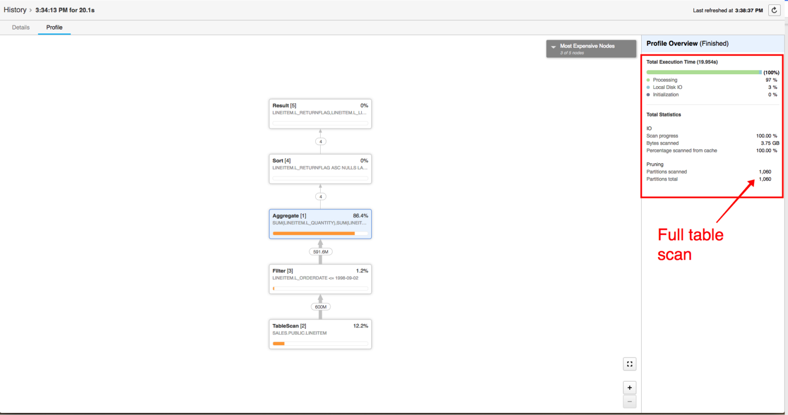
This query reports the amount of business that was billed, shipped and returned. If the developer has decided to issue a query against this table, we would see the following outcome in our query plan. (Note: the below result was performed on an XS warehouse):

It took about 19 seconds on an XS warehouse, which is not bad by any means. However, we can see that the query still performed a full table scan and performed a pretty good amount of aggregation.
Now, let’s see how we can improve the experience for the developer by creating a sample set of the LINEITEM table. We’ll create a special view (against our cloned dev database) for this developer and call it V_SALES_LINEITEM_SAMPLE_10. In this view, we’ll use the Block Sampling technique and only scan 10% of the partitions required by this query.
First create the view:
create view v_Sales_LineItem_Sample_10 as

   select *

   from SALES.PUBLIC.LINEITEM

   sample block (10);
Next, let’s update the query to use the view instead.
select

      l_returnflag,

      l_linestatus,

      sum(l_quantity) as sum_qty,

      sum(l_extendedprice) as sum_base_price,

      sum(l_extendedprice * (1 - l_discount)) as sum_disc_price,

      sum(l_extendedprice * (1 - l_discount) * (1 + l_tax)) as sum_charge,

      avg(l_quantity) as avg_qty,

      avg(l_extendedprice) as avg_price,

      avg(l_discount) as avg_disc,

      count(*) as count_order

 from

      v_Sales_LineItem_Sample_10

where

      l_orderdate <= dateadd(day, -90, to_date('1998-12-01'))

group by

      l_returnflag,

      l_linestatus

order by

      l_returnflag,

      l_linestatus;
Result:

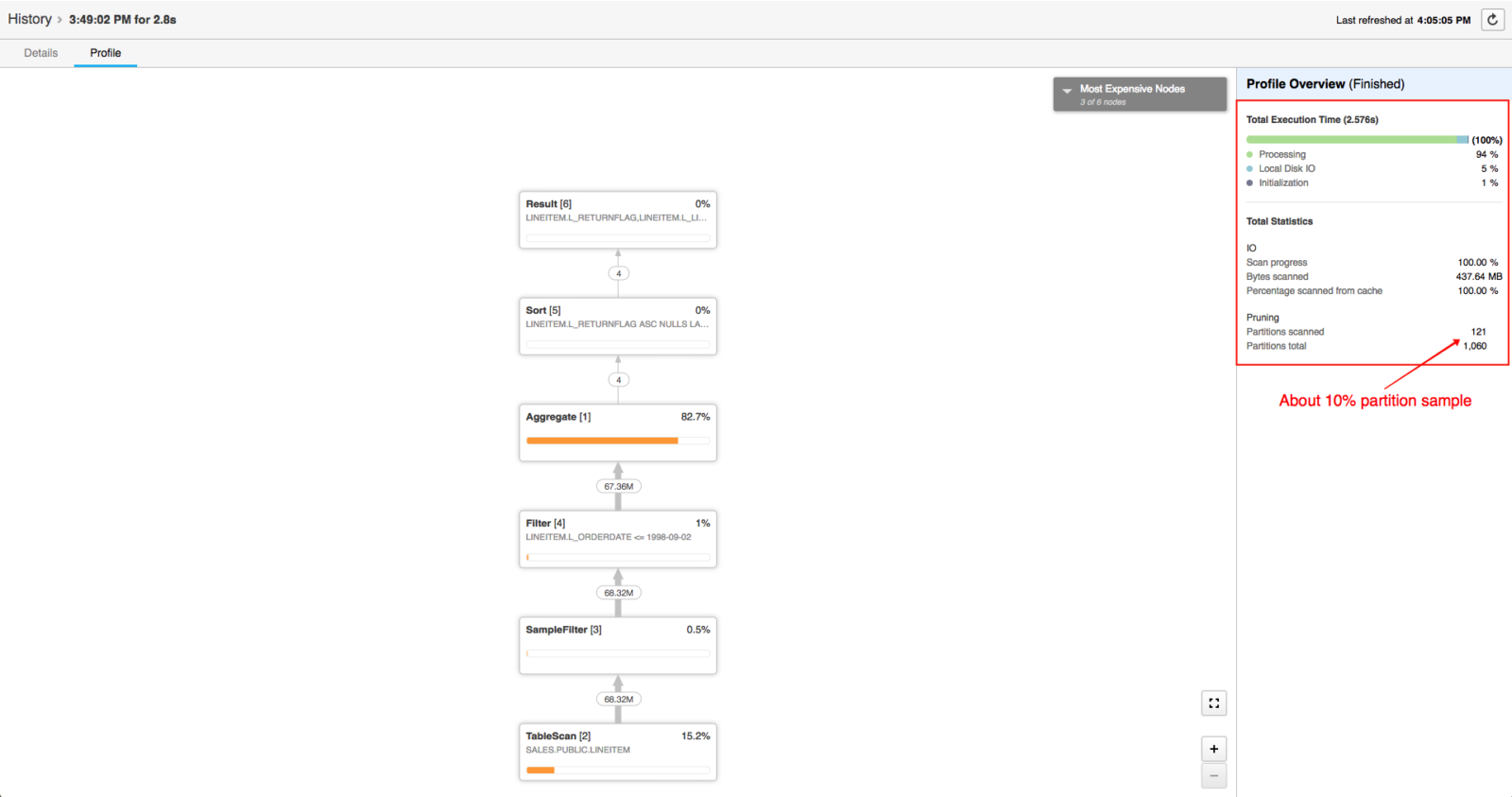
Let’s take a look at the query profile for this query:

This query ran about 2.5 seconds on an XS warehouse, and we scanned about 10% of the total table partition. This result is much better! Snowflake is sampling 10% of the partition to pull based on the WHERE filter. The result should still be accurate enough to let the developer know this query is working as expected.
In conclusion, leveraging Snowflake’s SAMPLE clause considerably reduces the amount of test dataset for a developer without losing data integrity. Even if a specific id or a timestamp biases the native data, chances are the developer is going to accept the nuance and continue with the development instead of spending additional compute credit and hours waiting for the results to return. The alternative is to use the LIMIT function perhaps to reduce the number of rows being returned. However, this involves modifying the original query or creating a view that still needs to be maintained. Using the SAMPLE clause, you can reliably subset a large table with acceptable result mix and performance. I hope you find this helpful. Feel free to leave comments in our community and let me know your thoughts.


