Simplify Spatial Indexing with the Power of H3 — What the World Needs Now Is a Hexagonal Grid

Did you know that approximately two thirds of Snowflake customers capture the latitude and longitude of some business entity or event in their account? While latitude and longitude columns can often be used by BI tools and Python libraries to plot points on a map, or shade common administrative boundaries such as states, provinces and countries, companies can do so much more with this valuable geospatial data to perform complex analyses. 

While we covered Snowflake’s support for GEOGRAPHY and GEOMETRY data types in this blog series, and millions of queries run daily using these types, the reality is that there are still many who feel they need to be a geospatial expert to work with them. They need an easier access path to convert that latitude and longitude into something more powerful. To paraphrase that old song from the 1960s, “What the world needs now” … is a hexagon.

We hear you, world. Today, we’re announcing the general availability of H3 in Snowflake. Now you can take your latitude and longitude data (and your GEOGRAPHY if you have it) and unlock the power of H3. But what is H3, and why does the world need a hexagon?

I love games of all kinds, specifically strategy games. A good strategy game will both challenge you within the constructs of the game, as well as force you to weigh your navigation within those constructs against the friends and family you are playing with. 

Strategy games come in a variety of styles, but there is one format I want to mention specifically: the tile placement game. In a tile placement game, players frequently have to place interconnecting tiles on a board or table to generate points or currency to win the game. There are many variations to this, but one theme that tile placement games often have is that they represent two-dimensional maps of a real or imaginary world. And because these tiles often need to perfectly connect with each other to build out or populate the map, the tiles often come in one of several shapes: a square, triangle or hexagon.

This process of placing shapes over a real or imaginary map in a game has parallels to the real world — we call it creating a spatial grid. A spatial grid attempts to organize a plane or sphere into many common shapes to be able to locate and reference each cell (shape) within that area faster. This grid, along with the metadata that represents the details of how the grid is constructed and used, is referred to as a spatial index. Snowflake partner CARTO notes that a spatial index can be a powerful tool because “they are geolocated by a short reference string, rather than a long geometry description which is much larger to store and slower to analyze.”

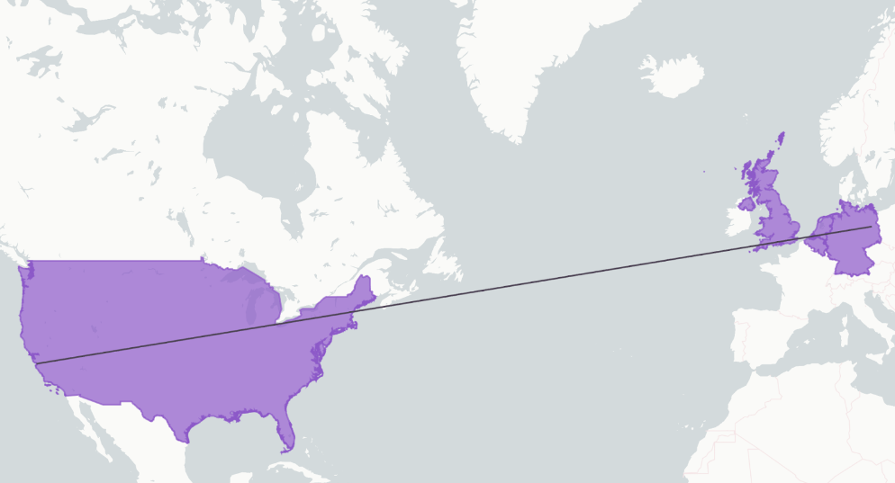
Uber, a popular rideshare company, had a need to optimize rideshare pricing and dispatch. They could have used standard government-defined polygons based on any number of existing levels of grouping within a municipality, but those are subject to change and are highly irregular. Consider the following image from part 2 of this blog series:

The polygons for the United States, Great Britain, Germany, the Netherlands and Belgium are highly irregular shapes. Their outlines require an incredibly dense series of points to render, and mathematical calculations against these polygons can be slow for some use cases. Uber needed the ability to represent a geographical area using a more uniform grid system that would allow fast calculations between predictable cells in the grid, so the company invented and eventually open sourced the spatial index H3.

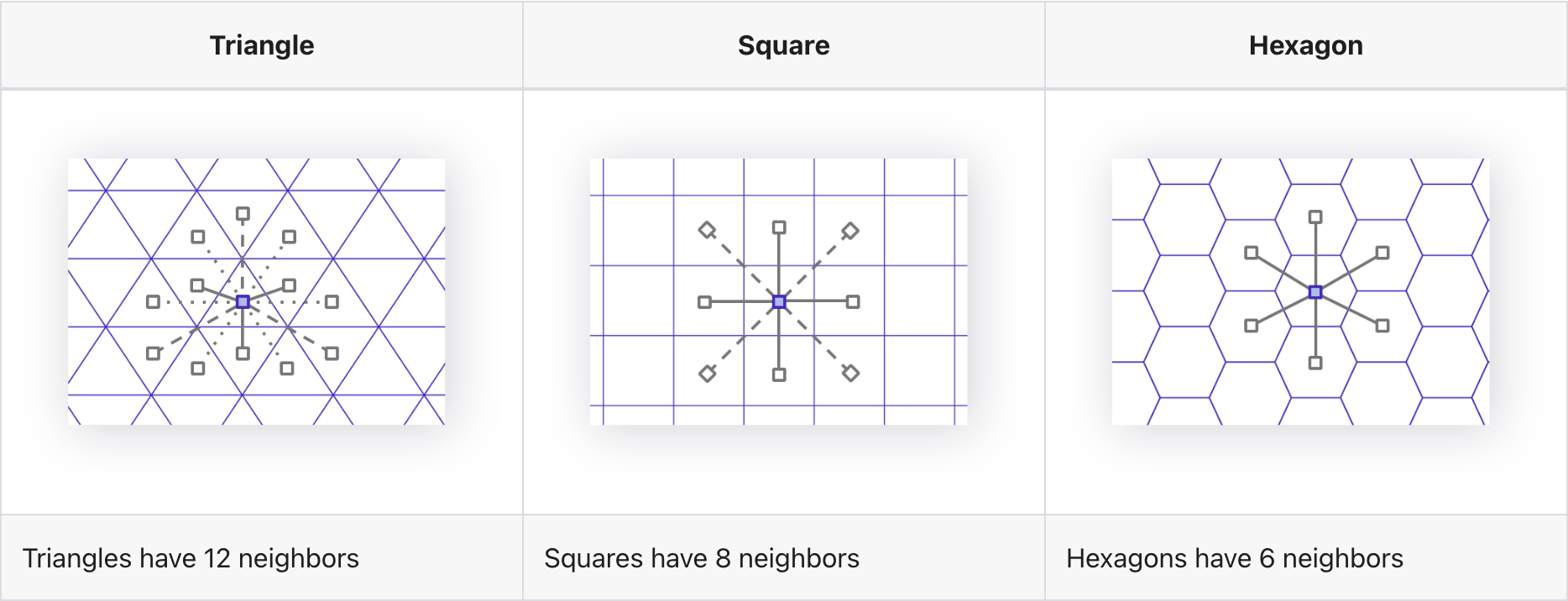
The first challenge was to determine what shape to use for their grid system. As I explained earlier, triangles, squares and hexagons are commonly used in a grid system because they interlock, or space-fill, very well. But hexagons have one important advantage over triangles and squares: they have equidistant neighbors:

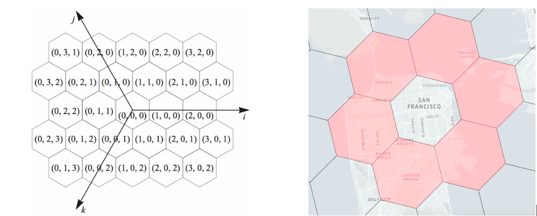
A hexagon within a grid has six neighboring hexagons whose centroids are a uniform distance apart from each other. This is not true for triangles or squares, making hexagons perfect for Uber’s geospatial use case because they could have a fast, singular distance category. This also allows for a simple coordinate system by creating a ring around a given hexagon:

The last element of H3 worth covering is the concept of resolution. Like video or TV resolution, which involves how many pixels are packed into a display or video file size, the grid system is designed with the concept of resolution to allow for different size hexagons to be used depending on the size of the area to be analyzed, or the granularity of the analysis required. This resolution is created as a hierarchy by layering one grid on top of another, with each layer having a slightly different orientation as shown below. When this is done correctly, seven hexagons centroids fit within a larger hexagon using a method called aperture 7, and there is a parent-child relationship created between the hexagons at every layer. Check different resolutions and play with hierarchy levels using the widget below.

Caption: A demo Streamlit app visualizes H3 hexagons at different resolutions for the same data.

There are 16 layers, or levels, of resolution in H3. In the demo Streamlit app below, you can see how cell tower concentration in the United States can be shown at different levels of resolution, which results in very different size hexagons:

Caption: A demo Streamlit app visualizes H3 hexagons at different resolutions for the same data.

But H3 isn’t just valuable for rideshare companies, it also works well for a number of use cases across a variety of industries:

• Telecoms: Network monitoring and planning. H3 enables the processing of massive network performance data volumes and the generation of unique customer usage insights.
• Insurance: Defining pricing strategies, and analyzing risk patterns against assets and infrastructure. 
• Sustainability and climate resilience analytics: Helping analysts to overcome the processing limitations and costs associated with handling and visualizing large raster data sets.
• Logistics and fleet management: Optimizing routings and delivery times, and better management of fleets at scale.
• Delivery and quick commerce: Evaluating business-critical performance indicators such as delivery delays and errors.

Caption: This map leverages H3 for the creation of a Wildfire Risk Index for California. Land cover type, temperature and wind speeds are all incorporated into one single score to help insurers understand the risk of wildfire. Source: CARTO

It’s easy to get started with H3 in Snowflake. Unlike GEOGRAPHY and GEOMETRY, H3 isn’t a data type. Instead, you use a collection of H3 functions with GEOGRAPHY data that is either stored in a GEOGRAPHY data type, or stored as discrete latitude and longitude columns. By using Streamlit in Snowflake and the PyDeck package, you can build dashboards that visualize this data.

The easiest set of functions to get started with is H3_[object]_TO_CELL, where [object] can either be a GEOGRAPHY POINT or a combination of latitude and longitude columns. These functions return the H3 cell id for a given object. There are two variations that work with either type of object, and there are two variations that return the H3 cell id in integer or hexadecimal format:

• H3_POINT_TO_CELL
• H3_POINT_TO_CELL_STRING
• H3_LATLNG_TO_CELL
• H3_LATLNG_TO_CELL_STRING

Whether you choose integer or hexadecimal depends on your use case. Hexadecimal is more broadly supported across visualization tools and libraries that support H3, but integers will be more efficient for storage, as well as join or aggregation performance. So choose the variation that best suits your use case.

You can see below that I have a table called ALL_NODES, which has a column S_GEOGRAPHY stored in the GEOGRAPHY data type. I also have a column TAGS, which I will use to isolate the location of the Eiffel Tower in Paris.

There are two things happening in the above query:

• First, we’re using both H3_POINT_TO_CELL (lines 2 & 3) and H3_POINT_TO_CELL_STRING (lines 4 & 5) to return the H3 cell id for the Eiffel Tower in both integer and hexadecimal representation, respectively.
• Second, both functions require a specific resolution. Remember that H3 actually has 16 layers of hexagonal grids, so to get the corresponding H3 cell id for a point, we need to know which resolution we want it at. In this case, we used resolutions 8 and 9.

But again, we don’t need data already stored in a GEOGRAPHY data type — we just need latitude and longitude columns. So let’s create a view of ALL_NODES called ALL_NODES_V, which extracts the latitude and longitude from the S_GEOGRAPHY column and stores them as separate columns. We can then replicate the above query below, substituting the appropriate columns from the new view and different functions:

There are two things to note in the above two queries:

• First, we’re switching to H3_LATLNG_TO_CELL (lines 14 & 15) and H3_LATLNG_TO_CELL_STRING (lines 16 & 17) functions, which use discrete latitude and longitude columns as arguments. Remember: two thirds of you already have this data in your Snowflake account!
• Second, notice that we get the exact same H3 cell ids in query 1 as we do in query 2.

These same transformation capabilities that exist for a POINT or a latitude/longitude combination also exist for a POLYGON. These functions allow you to overlay the H3 grid over your polygons, an action also known as polyfill. These functions behave a little differently, though: 

• H3_POLYGON_TO_CELLS is planar and does a centroid-based polyfill. This method will produce better results in more localized areas.
• H3_COVERAGE uses spherical geometry calculations and returns cells that fully cover a shape. It works well for data on a much larger scale.

The difference between these two polyfill approaches can be seen in the Streamlit app mentioned earlier:

Caption: A Streamlit app showing the difference between two different polyfill functions at different H3 resolutions.

Notice how H3_POLYGON_TO_CELLS doesn’t align well at the more global scale on the left, but it polyfills a little cleaner than H3_COVERAGE for the smaller area on the right.

There are another set of functions that let you navigate up and down the resolution hierarchy within H3. As noted before, the 16 layers all behave in a parent/child relationship. First, we find the parent of any given H3 cell id at a particular resolution using H3_CELL_TO_PARENT:

On lines 23 and 25 in the query above, we’re wrapping the H3_LATLNG_TO_CELL and H3_LATLNG_TO_CELL_STRING functions at resolution 9 with H3_CELL_TO_PARENT to give us the parent cell id at resolution 8. Leaving in the original resolution 8 columns on lines 22 and 24, we can see in the results how the values match. We could have also skipped resolution 8 and jumped to resolution 7 or lower, all the way down to resolution 0. A parent resolution number is always a lower number.

We can use the same type of function in reverse to find all of the child cells for a given parent cell. This function is named H3_CELL_TO_CHILDREN, and it goes in the opposite resolution direction: lower to higher. Let’s simplify the query a bit by removing a few columns because the results will look different from the previous queries:

Line 31 is asking for the children of a particular cell at resolution 9, and line 30 represents the Eiffel Tower cell at resolution 9. You can see how the children are returned in an array and there are seven of them. If we isolate that array in the sidebar, we can see that indeed the Eiffel Tower cell is one of the cells listed in the array (red highlight box).

This is all well and good, but we haven’t really done anything interesting yet. These functions are useful for transforming your geospatial data into H3, but once you’re there, what can you do with it? Let’s consult some outside help to go deeper.

Snowflake partner CARTO provides a wide range of features for deriving insights from spatial data.

One key feature is CARTO’s Analytics Toolbox, available as a Snowflake Native App from Snowflake Marketplace. This allows you to leverage advanced analytical procedures — from running statistical analyses such as Geographically Weighted Regression to enriching your H3 index with data from another enrichment query that contains geographies (such as administrative regions). These advanced stored procedures are accessible in Snowflake through the CALL command, and each procedure takes a set of arguments to make them easier to use than writing a series of large SQL statements by hand.

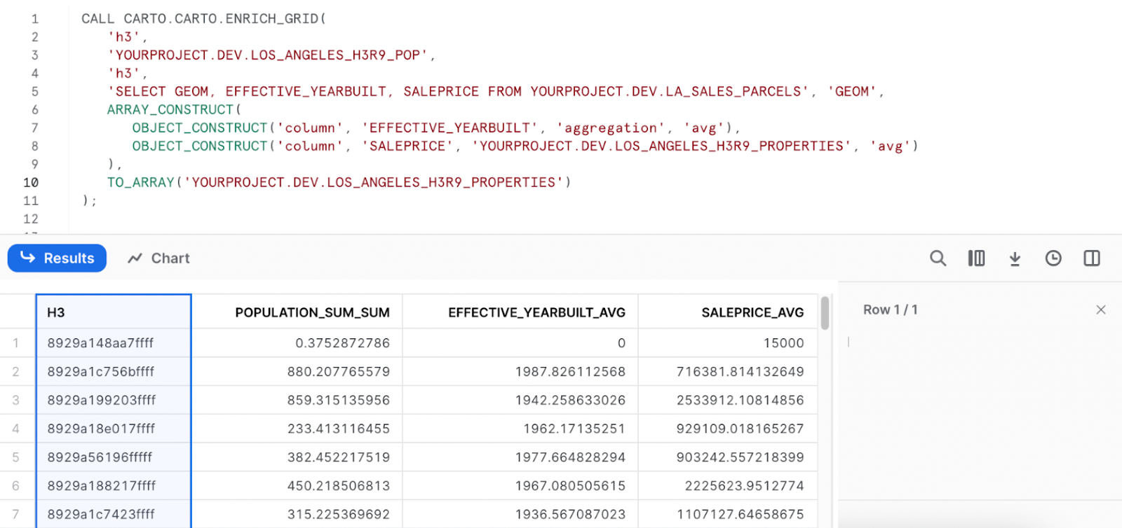
Let’s look at an example using the Analytics Toolbox procedure called ENRICH_GRID. This procedure aggregates columns from a source table based on the area which overlaps the target H3 table: 

In the example above, Los Angeles property data is aggregated to a H3 grid in the following steps:

1. Lines 2-4: The user specifies the target grid type (‘h3’), the target table (‘LOS_ANGELES_H3R9_POP’) and the target H3 column (‘h3’).
2. Line 5: the source table and geography column are specified (‘LA_SALES_PARCELS’ and ‘GEOM’ respectively).
3. Lines 6-9: an array is constructed specifying the columns to be aggregated and an aggregation method. In this example, both the year built (‘EFFECTIVE_YEARBUILT’) and property price (‘SALEPRICE’) are averaged.
4. Line 10: the output table is specified.

More information on this process can be found in the Analytics Toolbox documentation. 

Let’s look at the difference between visualizing the source table and the target table:

Caption: Maps in CARTO showing the difference between visualizing data via points vs H3. Source: carto.com.

We can see the results of this analysis on the maps above. The property parcels (source table) is on the left-hand map, with the resulting H3 aggregated grid (target table) on the right — both are showing the average sale price data. Note how much easier it is to interpret spatial patterns through the H3 grid, not to mention the data loads more quickly as you explore the map due to the speed of H3 calculations. CARTO progressively generates tiles on demand based on highly optimized SQL queries that are pushed down to your Snowflake database with a mechanism named Dynamic Tiling, and it’s able to directly translate the H3 indexes present in your data into the hexagonal cells that are rendered in the map.

Even if you aren’t a geospatial expert, you can expand the use of your latitude and longitude data by embracing the H3 spatial index. Using a combination of Snowflake and CARTO, you can power more performant and sophisticated analyses with more impactful visualizations to gain better insights into your business. If you want to learn more about H3, check out our geospatial documentation and our new Quickstart for performance optimization approaches with geospatial data. Join the live webinar hosted by CARTO on March 13 at 12 pm ET //5 pm CET, where we will share even more techniques and use cases.